Where Card(X) Is the Cardinality of the Vector X, Defined as the Number of Nonzero Elements in X
Introduction:
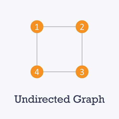
What is a graph? Do we use it a lot of times? Lease's dream up an exemplar: Facebook. The humongous network of you, your friends, family, their friends and their friends etc. are called as a multi-ethnic graph. In that "chart", every mortal is considered A a node of the graphical record and the edges are the links between two mass. In Facebook, a friend of yours, is a bidirectional relationship, i.e., A is B's Friend => B is A's friend, so the chart is an Undirected Chart.
Nodes? Edges? Undirected? We'll get to everything slowly.
Rent out's redefine graphical record by saying that it is a collection of finite sets of vertices Beaver State nodes (V) and edges (E). Edges are represented as ordered pairs (u, v) where (u, v) indicates that there is an edge from vertex u to vertex v. Edges may control toll, weight or distance. The degree or valency of a vertex is the number of edges that connect thereto. Graphs are of two types:
Undirected: Undirected graph is a graph in which all the edges are bidirectional, essentially the edges don't direct in a specific direction.
Directed: Directed graphical record is a chart in which all the edges are unidirectional. 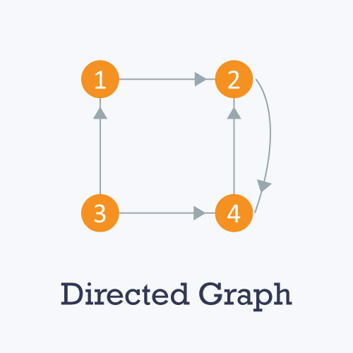
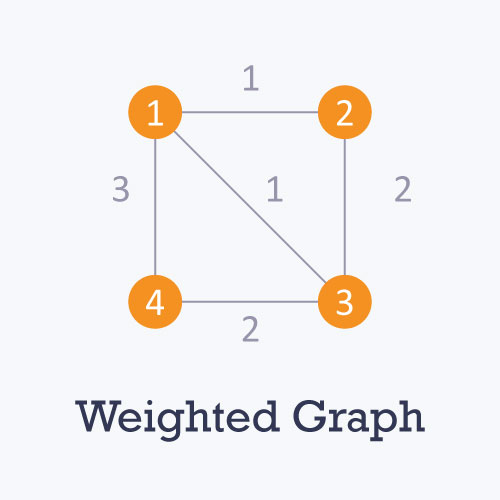
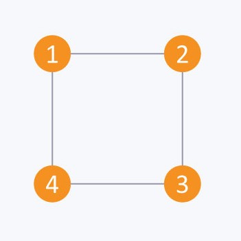
A weighted graph is the one in which each edge is appointed a weight or cost. Consider a graph of 4 nodes as shown in the diagram under. As you behind see each edge has a weight/monetary value assigned thereto. Suppose we need to go from vertex 1 to vertex 3. There are 3 paths.
1 -> 2 -> 3
1 -> 3
1 -> 4 -> 3
The total cost of 1 -> 2 -> 3 will be (1 + 2) = 3 units.
The total toll of 1 -> 3 will be 1 units.
The total be of 1 -> 4 -> 3 testament be (3 + 2) = 5 units.
A graph is called cyclic if there is a path in the graph which starts from a vertex and ends at the same peak. That path is called a cycle. An open-chain graph is a graph which has no oscillation.
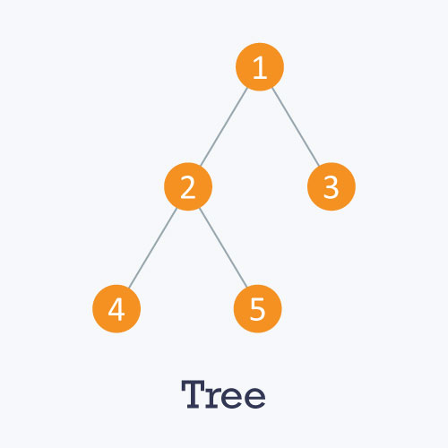
A tree is an undirected graph in which any two vertices are connected aside single cardinal path. Tree is acyclic chart and has N - 1 edges where N is the number of vertices.
Graph Histrionics:
There are variety of ways to represent a graph. Two of them are:
Adjacency Matrix: An adjacency matrix is a V x V binary matrix A (a binary intercellular substance is a matrix in which the cells rear have single one of two possible values - either a 0 or 1). Constituent Ai,j is 1 if there is an edge from acme i to vertex j else Ai,j is 0. The adjacency matrix can also embody modified for the adjusted chart in which instead of storing 0 or 1 in Ai,j we will store the weight or cost of the abut from vertex i to vertex j. In an undirected graph, if Ai,j = 1 then Aj,i = 1. In a directed graph, if Ai,j = 1 then Aj,i may operating room may not be 1. Adjacency ground substance providers continual time get at (O(1) ) to tell if there is an edge between two nodes. Space complexity of contiguity matrix is O(V2).
The adjacency matrix of to a higher place graph is:
i/j : 1 2 3 4
1 : 0 1 0 1
2 : 1 0 1 0
3 : 0 1 0 1
4 : 1 0 1 0
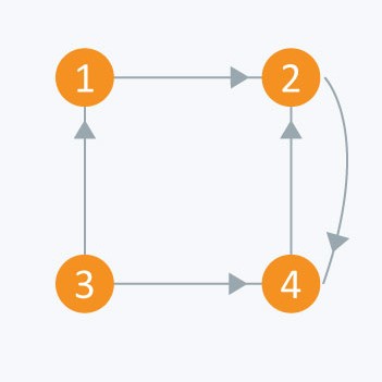
The adjacency matrix of above chart is:
i/j: 1 2 3 4
1 : 0 1 0 0
2 : 0 0 0 1
3 : 1 0 0 1
4 : 0 1 0 0
Consider the above directed graph and let America make this graph using an Adjacency ground substance and then show all the edges that exist in the graph.
Input File cabinet:
4
5
1 2
2 4
3 1
3 4
4 2
Code:
#include <iostream> victimization namespace std; bool A[10][10]; void initialize() { for(int i = 0;i < 10;++i) for(int j = 0;j < 10;++j) A[i][j] = false; } int main() { int x, y, nodes, edges; initialize(); // Since thither is no abut initially cin >> nodes; // Number of nodes cin >> edges; // Number of edges for(int i = 0;i < edges;++i) { cin >> x >> y; A[x][y] = true; // mark the edges from vertex x to vertex y } if(A[3][4] == sincere) cout << "There is an edge between 3 and 4" << endl; other cout << "In that respect is no edge betwixt 3 and 4" << endl; if(A[2][3] == true) cout << "There is an edge between 2 and 3" << endl; else cout << "There is no edge between 2 and 3" << endl; restoration 0; } Output:
Thither is an butt on between 3 and 4
There is no butt between 2 and 3
Adjacency List: The other means to represent a graph is an contiguity inclination. Contiguousness list is an array A of separate lists. To each one element of the array Ai is a list which contains all the vertices that are adjacent to vertex i. For weighted graph we dismiss store weight operating theatre cost of the butt against on with the vertex in the list using pairs. In an directionless graph, if acme j is in list Ai then vertex i will be in list Aj . Space complexity of adjacency list is O(V + E) because in Adjacency leaning we store information for only those edges that really subsist in the chart. In a lot of cases, where a matrix is sparse (A sparse matrix is a matrix in which most of the elements are zero in. By contrast, if most of the elements are nonzero, past the matrix is considered dense.) using an contiguity matrix power not be very useful, since it'll use much of space where all but of the elements will be 0, anyway. In such cases, using an adjacency list is better.

Consider the same undirected graph from adjacency intercellular substance. Adjacency list of the graphical record is:
A1 → 2 → 4
A2 → 1 → 3
A3 → 2 → 4
A4 → 1 → 3

Consider the same graph from adjacency ground substance. Contiguousness heel of the graph is:
A1 → 2
A2 → 4
A3 → 1 → 4
A4 → 2
Consider the above directed graph and let's cipher information technology.
Stimulation File:
4
5
1 2
2 4
3 1
3 4
4 2
Encode:
#include<iostream > #include < vector > using namespace std; vector <int> adj[10]; int main() { int x, y, nodes, edges; cin >> nodes; // Number of nodes cin >> edges; // Amoun of edges for(int i = 0;i < edges;++i) { cin >> x >> y; adj[x].push_back(y); // Insert y in adjacency list of x } for(int i = 1;i <= nodes;++i) { cout << "Adjacency list of lymph node " << i << ": "; for(int j = 0;j < adj[i].size of it();++j) { if(j == adj[i].size() - 1) cout << adj[i][j] << endl; else cout << adj[i][j] << " --> "; } } return 0; } Outturn:
Contiguousness inclination of lymph node 1: 2
Adjacency list of lymph gland 2: 4
Adjacency listing of node 3: 1 --> 4
Adjacency tilt of node 4: 2
Graph Traversals:
Patc using any graph algorithms, we need that every vertex of a graph should be visited incisively once. The set up in which the vertices are visited may be great, and may depend on the particular algorithmic rule or fussy question which we're trying to solve. During a traversal, we must continue track of which vertices have been visited. The most common way is to mark the vertices which have been visited.
So, graph traversal means visiting all vertex and every margin incisively once in more or less easily-defined social club. There are many approaches to traverse the graph. Cardinal of them are:
Depth First Search (DFS):
Depth first search is a algorithmic algorithmic program that uses the theme of backtracking. Basically, it involves exhaustive searching of all the nodes by going ahead - if IT is possible, other than information technology will backtrack. By double back, Here we mean that when we do not get any further node in the current path then we move back to the node,from where we can find the promote nodes to traverse. In different wrangle, we will continue visiting nodes A soon as we find an unvisited node connected the current path and when current path is altogether traversed we will select the close route.
This recursive nature of DFS can be implemented victimization stacks. The standard idea is that we pick a start node and push all its adjacent nodes into a stack. And then, we pop a node from stack to select the succeeding client to visit and push completely its adjacent nodes into a batch. We keep connected repeating this process until the hatful is empty. But, we do not visit a node much once, otherwise we might end up in an innumerous closed circuit. To avoid this infinite loop, we will gull the nodes as soon as we visit it.
Pseudocode :
DFS-iterative (G, s): //where G is graph and s is source vertex. let S be stack S.push( s ) // inserting s in stack stain s as visited. while ( S is non empty): // soda water a vertex from stack to visit next v = S.top( ) S.crop up( ) //push all the neighbours of v in raft that are not visited for all neighbours w of v in Graph G: if w is non visited : S.push( w ) mark w as visited DFS-recursive(G, s): mark s as visited for every last neighbours w of s in Graph G: if w is non visited: DFS-recursive(G, w) 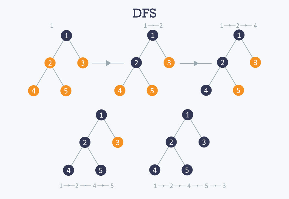
Applications:
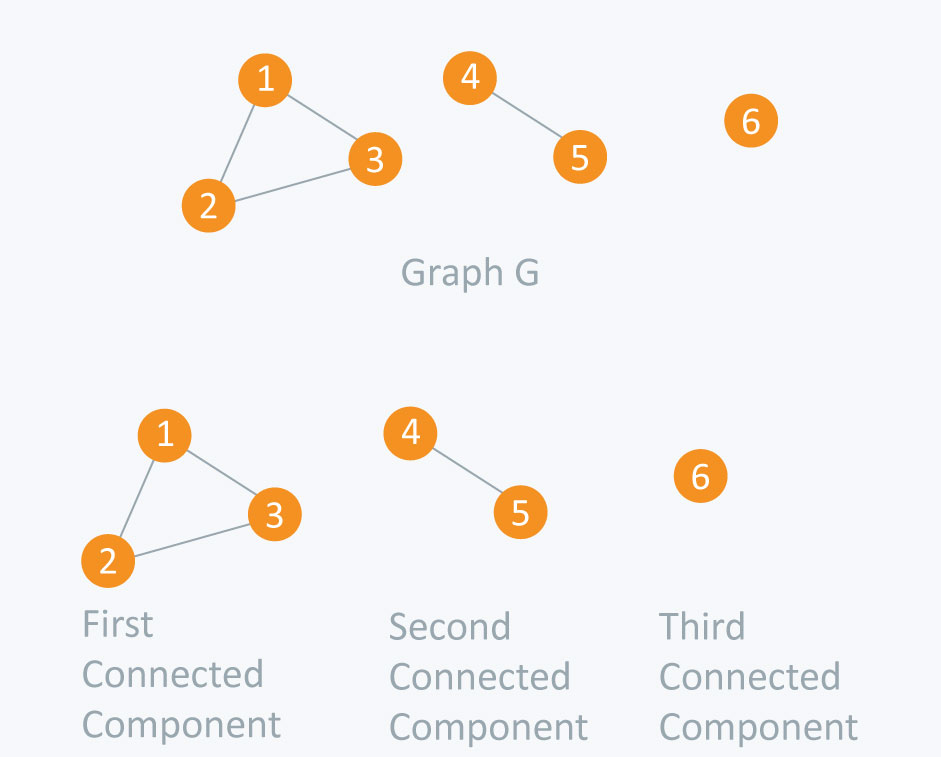
1) How to find connected components using DFS?
A graph is aforementioned to be disconnected if it is not connected, i.e., if there exist two nodes in the graph so much that there is no edge 'tween those nodes. In an undirected graph, a connected component is a mark of vertices in a graph that are linked to apiece other aside paths. Consider an representative inclined in the diagram. As we can see graph G is a disconnected graph and has 3 engaged components. First connected component is 1 -> 2 -> 3 as they are linked to each other. Second connected component 4 -> 5 and third connected component is vertex 6. In DFS, if we set forth from a start node information technology bequeath mark all the nodes connected to offse lymph node as visited. Then if we choose any node in a coupled part and run DFS thereon node it wish mark the wholly affiliated component as visited. So we will repeat this process for other connected components.
Input data:
6
4
1 2
2 3
1 3
4 5
Code:
#include <iostream> #admit <vector> using namespace std; vector <int> adj[10]; bool visited[10]; void dfs(int s) { visited[s] = true; for(int i = 0;i < adj[s].size of it();++i) { if(visited[adj[s][i]] == delusive) dfs(adj[s][i]); } } void format() { for(int i = 0;i < 10;++i) visited[i] = false; } int main() { int nodes, edges, x, y, connectedComponents = 0; cin >> nodes; // Number of nodes cin >> edges; // Numeral of edges for(int i = 0;i < edges;++i) { cin >> x >> y; // Planless Graph adj[x].push_back(y); // Edge from apex x to vertex y adj[y].push_back(x); // Adjoin from vertex y to peak x } initialize(); // Initialize all nodes atomic number 3 not visited for(int i = 1;i <= nodes;++i) { if(visited[i] == false) { dfs(i); connectedComponents++; } } cout << "Numerate of adjoining components: " << connectedComponents << endl; return 0; } Output:
Number of on-line components: 3
Largeness First Search (BFS)
Its a traversing algorithm, where we start traversing from selected lymph node (source or starting knob) and traverse the chart layerwise which means IT explores the neighbour nodes (nodes which are right away connected to source knob) and and then move towards the next level neighbour nodes. As the name suggests, we draw in width of the graphical record, i.e., we move horizontally first and visit all the nodes of the underway layer and then we move to the side by side layer.
Consider the diagram below:
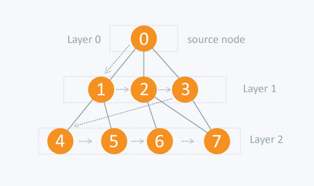
In BFS, all nodes on layer 1 will be traversed earlier we move to nodes of layer 2. As the nodes on stratum 1 have less distance from source node when compared with nodes happening layer 2.
As the graph can contain cycles, so we may come at same node again while traversing the graph. So to avoid processing of same node again, we use a boolean array which marks the lymph node marked if we have unconscious process that node. While visiting all the nodes of current layer of graph, we will store them in such a way, so that we bathroom visit the children of these nodes in the same order as they were visited.
In the above diagram, protrusive from 0, we will jaw its children 1, 2, and 3 and storage them in the order they obtain visited. So that after visiting totally the vertices of current layer, we can visit the children of 1 forward(that are 4 and 5), then of 2 (that are 6 and 7) and then of 3(that is 7) and then along.
To make the above process easy, we volition use a queue to salt away the knob and mark it as visited, and we will store information technology in queue until every its neighbours (vertices which are like a shot siamese to that) are marked. As queue follow FIFO order (Freshman In First Unstylish), IT will first visit the neighbours of that node, which were inserted ordinal in the queue.
Pseudocode :
BFS (G, s) //where G is graph and s is source node. let Q embody line up. Q.enqueue( s ) // inserting s in queue until whol its neighbour vertices are noticeable. mark s as visited. piece ( Q is not empty) // removing that vertex from queue,whose neighbor will be visited now. v = Q.dequeue( ) //processing totally the neighbours of v for all neighbours w of v in Chart G if w is non visited Q.enqueue( w ) //stores w in Q to further visit its neighbour Deutsche Mark w as visited. For the Chart below: 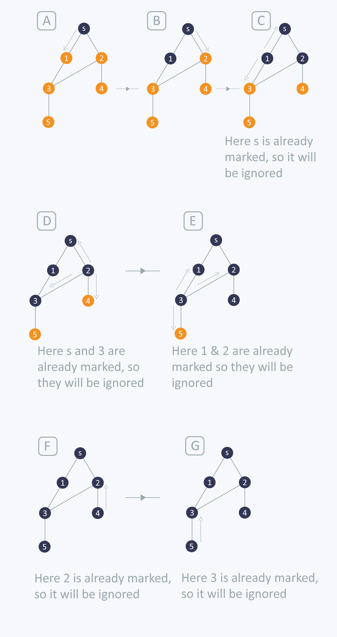
Initially, it bequeath start from the source node and will push s in queue and note s American Samoa visited.
In first looping, It will pop s from queue and then will deny on neighbours of s that are 1 and 2. Arsenic 1 and 2 are unvisited, they will be pushed in queue and will be conspicuous as visited.
In second looping, it will pop 1 from queue so will traverse on its neighbours that are s and 3. As s is already marked so it will be ignored and 3 is pushed in queue and marked as visited.
In third iteration, it will pop 2 from queue and then will traverse happening its neighbours that are s,3 and 4. As 3 and s are already marked sol they will be ignored and 4 is pushed in queue up and marked as visited.
In fourth iteration, information technology will pop 3 from queue and and then will traverse on its neighbours that are 1, 2 and 5. As 1 and 2 are already noticeable so they will be ignored and 5 is pushed in queue and marked as visited.
In fifth iteration, it leave soda pop 4 from queue and so will sweep happening its neighbours that is 2 only. Eastern Samoa 2 is already marked so information technology will be ignored.
In sixth iteration, information technology volition pop music 5 from line up and then will traverse happening its neighbours that is 3 only. As 3 is already marked so information technology leave be neglected.
Now the queue up is empty so information technology comes out of the loop.
Through this you tin can traverse all the nodes using BFS.
BFS can be used in finding minimum length from one lymph gland of graphical record to another, provided every last the edges in graphical record have like weight.
Example:
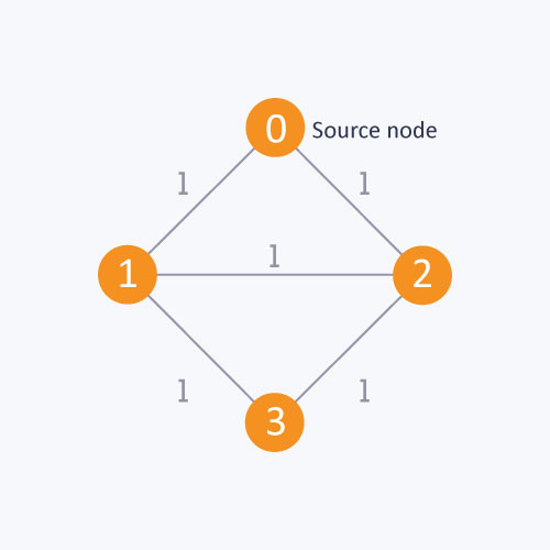
As in the above diagram, starting from rootage lymph gland, to find the distance 'tween 0 and 1, if we do not follow BFS algorithm, we backside go from 0 to 2 so to 1. It will give the aloofness between 0 and 1 as 2. Merely the tokenish distance is 1 which can be obtained by using BFS.
Complexness: Time complexity of BFS is O(V + E) , where V is the number of nodes and E is the number of Edges.
Applications:
1) How to determine the level of each node in the given tree ?
Every bit we know in BFS, we sweep level wise, i.e first-year we visit all the nodes of one level and then visit to nodes of other level. We can use BFS to mold level of each client.
Implementation:
transmitter <int> v[10] ; // vector for maintaining adjacency name explained above. int level[10]; // to determine the level of each node bool vis[10]; //St. Mark the node if visited void bfs(int s) { queue <int> q; q.agitate(s); level[ s ] = 0 ; //setting the steady of sources node as 0. vis[ s ] = true; while(!q.devoid()) { int p = q.front(); q.pop(); for(int i = 0;i < v[ p ].size of it() ; i++) { if(vis[ v[ p ][ i ] ] == false) { //setting the level of each node with an increment in the steady of parent client level[ v[ p ][ i ] ] = level[ p ]+1; q.agitate(v[ p ][ i ]); vis[ v[ p ][ i ] ] = true; } } } } In a higher place code is similar to bfs except one change and i.e
level[ v[ p ][ i ] ] = pull dow[ p ]+1;
here, when visiting each node, we set the level of that lymph gland with an increment in the floor of its raise node .
Through this we can determine the level of each node.
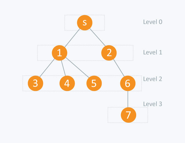
In the diagram above :
thickening level[ node ] s(source node) 0 1 1 2 1 3 2 4 2 5 2 6 2 7 3 2) 0-1 BFS: This type of BFS is used when we take over to find the shortest distance from one guest to another in a chart provided the edges in graph have weights 0 or 1. As if we apply the formula BFS explained preceding, it can give inopportune results for optimal distance between 2 nodes.(explained to a lower place)
In this approach we will not use Boolean align to mark the knob visited as piece visiting for each one node we will check the condition of optimum distance.
We will use Double All over Queue to store the node.
In 0-1 BFS, if the edge is encountered having weight = 0, and then the node is pushed to foremost of dequeue and if the edge's weight =1, then IT will be pushed to back of dequeue.
Effectuation:
Here :
edges[ v ] [ i ] is an adjacency lean that will exists in yoke form i.e edges[ v ][ i ].first will contains the number of node to which v is adjunctive and edges[ v ][ i ].moment volition stop the distance between v and edges[ v ][ i ].first .
Q is double ended queue.
distance is an array where, distance [ v ] will hold back the distance from start thickening to v lymph gland.
Initially define aloofness from source lymph gland to each node Eastern Samoa infinity.
void bfs (int start) { deque <int > Q; // double ended waiting line Q.push_back( start); distance[ bug out ] = 0; while( !Q.empty ()) { int v = Q.frontal( ); Q.pop_front(); for( int i = 0 ; i < edges[v].size(); i++) { /* if distance of neighbour of v from originate in client is greater than sum of aloofness of v from start node and margin burden between v and its neighbor (distance between v and its neighbour of v) ,then change it */ if(distance[ edges[ v ][ i ].first ] > outstrip[ v ] + edges[ v ][ i ].second ) { distance[ edges[ v ][ i ].first ] = distance[ v ] + edges[ v ][ i ].second; /*if edge weight unit between v and its neighbour is 0 then push it to front of double ended queue else push it to back*/ if(edges[ v ][ i ].secondment == 0) { Q.push_front( edges[ v ][ i ].first); } else { Q.push_back( edges[ v ][ i ].freshman); } } } Let's understand the preceding code with the Graph given below:
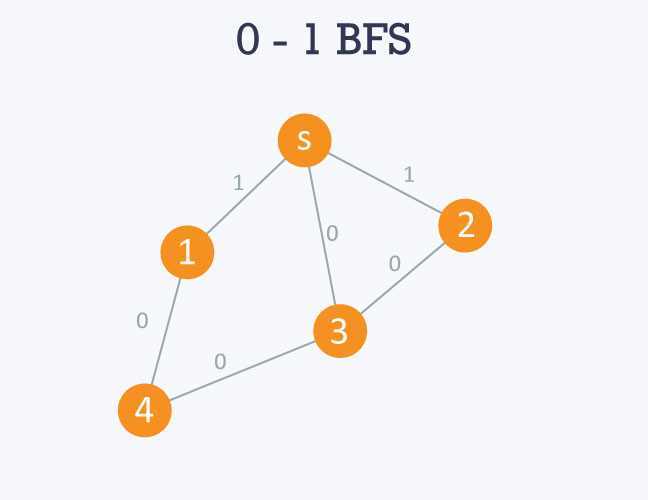
Adjacency List of to a higher place graph will glucinium:
here s can be taken as 0 .
0 -> 1 -> 3 -> 2
edges[ 0 ][ 0 ].first = 1 , edges[ 0 ][ 0 ].back = 1
edges[ 0 ][ 1 ].first = 3 , edges[ 0 ][ 1 ].second = 0
edges[ 0 ][ 2 ].low = 2 , edges[ 0 ][ 2 ].second = 1
1 -> 0 -> 4
edges[ 1 ][ 0 ].first = 0 , edges[ 1 ][ 0 ].secondly = 1
edges[ 1 ][ 1 ].first = 4 , edges[ 1 ][ 1 ].indorse = 0
2 -> 0 -> 3
edges[ 2 ][ 0 ].first = 0 , edges[ 2 ][ 0 ].second gear = 0
edges[ 2 ][ 1 ].first = 3 , edges[ 2 ][ 1 ].second = 0
3 -> 0 -> 2 -> 4
edges[ 3 ][ 0 ].first = 0 , edges[ 3 ][ 0 ].irregular = 0
edges[ 3 ][ 2 ].first = 2 , edges[ 3 ][ 2 ].second = 0
edges[ 3 ][ 3 ].first = 4 , edges[ 3 ][ 3 ].second = 0
4 -> 1 -> 3
edges[ 4 ][ 0 ].firstly = 1 , edges[ 4 ][ 0 ].second = 0
edges[ 4 ][ 1 ].first = 3 , edges[ 4 ][ 1 ].second = 0
So if we function modal bfs here, it will have U.S. wrong results by showing optimal distance between s and 1 node as 1 and betwixt a and 2 American Samoa 1, just the echt optimal distance is 0 in some the cases. As information technology simply visits the children of s and calculate the distance between s and its children which will give 1 as the answer.
Processing:
Initiating from source node, i.e 0, it testament movement towards 1,2 and 3. As the edge weight 'tween 0 and 1 is 1 and between 0 and 2 is 1 , so they bequeath equal pushed in back side of queue up and every bit march weight betwixt 0 and 3 is 0, so it will pushed in look side of queue. Accordingly, distance will be maintained in distance array.
Then 3 will be popped in the lead from queue and same process will be applied on its neighbours and thus on..
3) Peer to Peer Networks: In peer to peer networks, Breadth For the first time Search is wont to find all neighbour nodes.
4) GPS Navigation systems: Breadth First Search is used to bump all neighboring locations.
5) Broadcasting in Network: In networks, a broadcasted bundle follows Breadth Number 1 Search to reach all nodes.
Where Card(X) Is the Cardinality of the Vector X, Defined as the Number of Nonzero Elements in X
Source: https://www.hackerearth.com/practice/notes/graph-theory-part-i/
0 Response to "Where Card(X) Is the Cardinality of the Vector X, Defined as the Number of Nonzero Elements in X"
Publicar un comentario